Statistical error model

Coverage and pairwise allele frequency comparisons

Code

# load dependencies
library(ggplot2)
library(tidyverse)

── Attaching packages ─────────────────────────────────────── tidyverse 1.3.2 ──
✔ tibble  3.1.8      ✔ dplyr   1.0.10
✔ tidyr   1.2.1      ✔ stringr 1.4.1 
✔ readr   2.1.3      ✔ forcats 0.5.2 
✔ purrr   0.3.4      
── Conflicts ────────────────────────────────────────── tidyverse_conflicts() ──
✖ dplyr::filter() masks stats::filter()
✖ dplyr::lag()    masks stats::lag()

Code

library(purrr)
library(cowplot)
set.seed(172452)

Simulate a pairwise comparison between alleles at a single location with coverage error. To do this, we use a random binomial distribution that takes in coverage and true allele frequency and outputs the estimated allele frequency.

Code

# how to simulate coverage
## rbinom(1, cvg, AFtrue) / cvg
## output is estimated AF

cvg <- 20
trueAF <- 0.43

estAF <- rbinom(1,cvg,trueAF) / cvg
estAF

[1] 0.45

Function that calculates estimated allele frequency when it is given coverage and true allele frequency:

Code

# function calculating estimated allele frequency
estAF <- function(cvg,trueAF){
  est <- rbinom(1,cvg,trueAF) / cvg
  return(est)
}

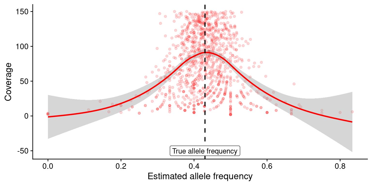
Now, we can scale our code and plot the results:

Code

# run this n times, scale up 
n <- 1000
tru <- 0.43
cvg <- sample(2:150,n,replace = TRUE)
af <- tibble(
  "cvg" = cvg,
  "trueAF" = rep(tru,times=n)
)

af$estAF <- af %>% pmap(estAF) %>% unlist()

# plot estimated allele frequency by coverage
plt <- af %>% ggplot(aes(x = estAF, y = cvg)) +
  geom_point(alpha = 0.15,colour="red") +
  geom_smooth(method = "gam", colour = "red") +
  geom_vline(xintercept=tru, size = 0.8,linetype = "dashed") +
  labs(x = "Estimated allele frequency", y = "Coverage") +
  annotate("label",x = tru, y = -50, label = "True allele frequency") +
  theme_cowplot()
plt

Figure 1: Variability in allele frequency estimations due to coverage.